深入理解transformer

transformer背景

主要内容

• 主要内容
  • attention设计原理解读
  • tranformer中的矩阵/行向量乘法
  • transformer的pytorch代码实现
  • 计算量\(O(N^2)\) 源于softmax的存在
  • 从kernel的角度来看attention
    • \(\mathcal{A}(X_i) = \dfrac{\sum_{j=1}^{N} sim(Q_i,K_j) V_j}{\sum_{j=1}^N sim(Q_i,K_j)}\)
    • linear attention
• 参考
  • 2017. Attention Is All You Need (Vaswani et al. 2023)
  • 2020. Fast Autoregressive Transformers with Linear Attention (Katharopoulos et al. 2020)
  • mingpt by karpathy

回顾线性代数的知识

why

• 原文比较晦涩 \[\begin{aligned}\mathrm{Attention}(Q,K,V)=\mathrm{softmax}(\dfrac{QK^T}{\sqrt{d_k}})V \\ \mathrm{MultiHead}(Q,K,V)=\mathrm{Concat}(\mathrm{head}_1,\ldots,\mathrm{head}_h)W^{O} \\ \mathrm{head}_i=\mathrm{Attention}(QW_i^Q, KW^{K}_i,VW^V_i) \end{aligned}\]
• 把矩阵剖解成从行向量来看更容易理解

矩阵和行向量

• 矩阵 \(X\in R^{N\times F}\) \(X=\begin{pmatrix} X_{11}, X_{12},\ldots, X_{1F} \\ X_{21}, X_{22},\ldots, X_{2F} \\ \vdots\\ X_{N1}, X_{N2},\ldots, X_{NF} \end{pmatrix}\)
• 行向量 \(X_{i}=\begin{pmatrix} X_{i1}, X_{i2},\ldots, X_{iF}\end{pmatrix}, X_i \in R^{1\times F}\)
• 分块矩阵 \(X=\begin{pmatrix} X_1\\ X_2\\ \vdots\\ X_N \end{pmatrix}\)
• 比如nn.Embedding 按照行向量来组织数据

1
2
3
4
5
6
7
8

import torch
import torch.nn as nn
N = 3
F = 8
embed = nn.Embedding(N, F)
idx = torch.tensor([1,2,3])
X = embed(idx)
print(X.shape)

• 例子

  • \(N\) 个token，\(F\) 是embedding的维度

  • 每行对应于一个token的embedding 行向量

    \(tokens=\begin{pmatrix} \text{hello} \\ \text{world} \\ \text{pad} \\ \text{pad} \\ \text{pad} \end{pmatrix}\)

    \(X=\begin{pmatrix} [0.59, 0.20, 0.04, 0.96] \\ [0.96, 0.30, 0.16, 0.63] \\ [0.02, 0.19, 0.34, 0.25] \\ [0.02, 0.19, 0.34, 0.25] \\ [0.02, 0.19, 0.34, 0.25] \end{pmatrix}\)

矩阵相乘和算子作用

• 定义线性算子 \(\mathcal{A}\)
  • 可以作用到行向量 \(\mathcal{A}(X_i) = X_{i} A\)
  • 也可以作用到矩阵 \(\mathcal{A}(X) = XA\)
• 右乘矩阵等于对每个行向量逐个施加行变换 \(XA=\begin{pmatrix} X_1\\ X_2\\ \vdots\\ X_N \end{pmatrix}A= \begin{pmatrix} X_1 A\\ X_2 A\\ \vdots\\ X_N A \end{pmatrix}= \begin{pmatrix} \mathcal{A}(X_1) \\ \mathcal{A}(X_2) \\ \vdots\\ \mathcal{A}(X_N) \end{pmatrix}=\mathcal{A}(X)\)
• 代码对应于 nn.Linear

1
2
3
4
5
6
7
8

import torch
import torch.nn as nn
F = 6
linear = nn.Linear(in_features=F, out_features=F)
X_i = torch.rand(1, 6)
X = torch.rand(3, 6)
print(linear(X_i).shape)
print(linear(X).shape)

• pytorch/tensorflow中的代码都是按照作用于行向量来组织的

从分块矩阵的乘法来看\(QK^{T}V\)

• \(S=QK^T\) 行向量两两计算点积相似性

  \(\begin{pmatrix} Q_{1}\\ Q_{2}\\ \vdots\\ Q_N \end{pmatrix} \begin{pmatrix} K_{1}^T, K_2^T,\ldots,K_N^T\\ \end{pmatrix}=(Q_{i}K_j^T)_{ij}=S\)

• \(SV\) = 对行向量做加权求和

  \(\begin{pmatrix} S_{11},S_{12},\ldots, S_{1N}\\ S_{21},S_{22},\ldots, S_{2N}\\ \vdots\\ S_{N1},S_{N2},\ldots, S_{NN}\\ \end{pmatrix} \begin{pmatrix} V_{1}\\ V_{2}\\ \vdots\\ V_N \end{pmatrix}= \begin{pmatrix} \sum\limits_{j}S_{1j}V_j\\ \sum\limits_{j}S_{2j}V_j\\ \vdots\\ \sum\limits_{j}S_{Nj}V_j \end{pmatrix}\)

• 基于Q,K计算相似性，然后基于V来加权求和

• \(QK^{T}V\) 的每个行向量都是\(V\) 行向量的一个加权求和

注

• 左乘以一个矩阵相当于对每个列向量来施加变化
• 论文：一般会有行/列向量两种表示方式
• 代码：基本都是行向量来作为数据组织的标准
• 本文:
  • 向量都按照行向量的形式来组织
  • 按照作用于单个行向量的方式来讲解transformer

encoder-decoder

• 大部分的s2s 的任务建模为 encoder-decoder的结构
  • 机器翻译，语音识别，文本摘要，问答系统等
• encoder
  • 把token序列\((x_{1}, x_2,\ldots, x_N)\) 转化为语义向量序列 \((Y_{1}, Y_2, \ldots, Y_N)\)
  • 一般组织为多层的网络的形式
    • 第一层：基础语义向量序列 \((x_{1}, x_2,\ldots, x_N)\rightarrow (X_{1}, X_2,\ldots, X_N)\)
    • 其它层：从低阶语义向量转化为高阶语义向量序列 \((X_{1}, X_2,\ldots, X_N)\rightarrow (Y_{1}, Y_2,\ldots, Y_N)\)
• decoder 基于\((Y_{1}, Y_2, \ldots, Y_N)\) 自回归式的逐个token解码

focus到 encoder部分来理解transformer

低阶到高阶语义向量的转换

encoder的主要工作是寻找算子\(\mathcal{T}\) 将低阶的语义向量序列变换为高阶的语义向量序列 \(\mathcal{T}\begin{pmatrix} X_1\\ X_2\\ \vdots\\ X_N \end{pmatrix} \rightarrow\begin{pmatrix} Y_1\\ Y_2\\ \vdots\\ Y_N \end{pmatrix}\)

• 输入: \(X\) 低阶语义向量序列，输出: \(Y\) 高阶语义向量序列
• 意义
  • \(Y_{i}=f(X_{1}, X_2, \ldots, X_{N})\)
  • 对低阶语义向量做加工组合处理和抽象，变换为一个高阶的语义向量序列
  • 高阶语义向量考虑了 上下文 的语义向量表达
• motivation
  • 1957. Firth

    a word is characterized by the company it keeps.

    例子：

    The enigmatic smile on Mona Lisa’s face has intrigued art enthusiasts for centuries, leaving them to speculate about its true meaning.

• 用算子作用来表达 \(Y=\mathcal{T}(X)\)
  • \(X \in R^{N\times F}\), \(Y=\mathcal{T}(X): \quad R^{N\times F}\rightarrow R^{N\times F}\)
  • 这个算子天然可以复合嵌套，形成多层的网络结构 \(Y=\mathcal{T}_{L}\circ \mathcal{T}_{L-1}\circ \ldots \circ \mathcal{T}_{1}(X)\)

核心的问题

问题

如何设计 \(Y_{i}=f(X_{1}, X_2, \ldots, X_{N})\)

• \(Y_{1}, \ldots, Y_N\) 能否并行得到
• \(Y_{i}\) 能否高效的建立起对周围token的远程依赖

RNN

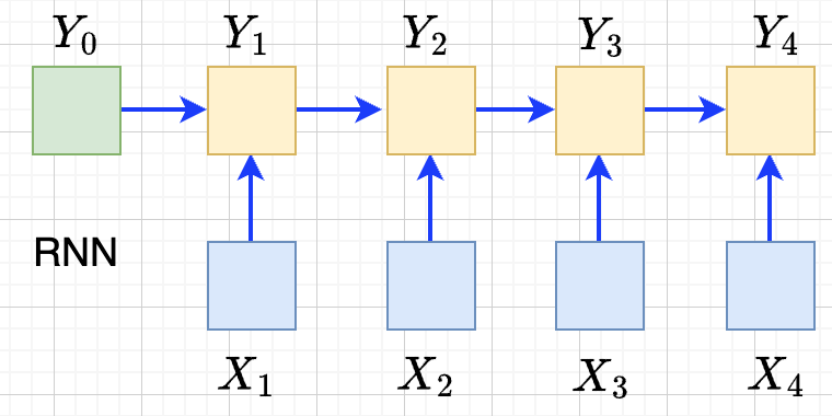
• 递归语义序列 \(Y_{0}\rightarrow Y_1 \rightarrow \ldots \rightarrow Y_{N}\)
• \(Y_{i}=tanh(X_{i}W + Y_{i-1}U)\)
• 串行
• 单方向的依赖关系 \(Y_{3}\) 直接依赖于\(Y_{2}, X_{3}\), 间接依赖于\(X_1\)

CNN

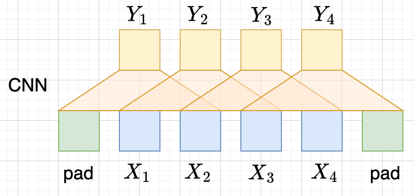
• \(Y_{i}=(X_{i-1},X_i, X_{i+1}) W\) 假设窗口宽度是3
• 并行
• 长距离依赖？
  • 一层卷积只能依赖于当前窗口内，不能对窗口外的形成依赖。

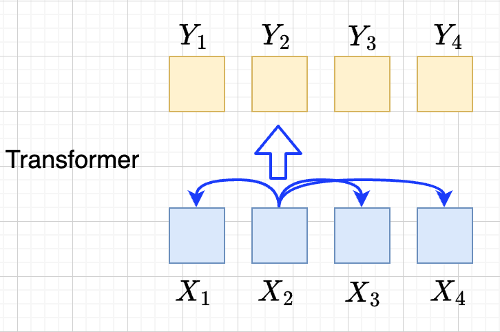
transformer思路

设计\(Y_{i}=f(X_{1}, X_2, \ldots, X_{N})\)，使得

• 使得 \(Y_{1},\ldots, Y_N\) 可以做并行计算
• 同时解决长距离依赖的问题

\(Y=\mathcal{F}\circ \mathcal{A}(X)\) 做两次矩阵的变换

• \(Y=\mathcal{A}(X)\) MultiHead Attention

  • 高阶的语义等于对 全部 的低阶语义向量基于 相似性(Attention) 做 加权平均
  • \(\begin{aligned}\mathcal{A}(X_i) &= \frac{\sum_{j=1}^{N} sim(X_i,X_j) X_j}{\sum_{j=1}^N sim(X_i,X_j)} \end{aligned}\)
  • attention = 相似性

• \(Y’=\mathcal{F}(Y)\) Position-wise Feedforward

  • 再施加若干非线性变换

tranformer网络结构

基于KV查询的相似性计算

\[\begin{aligned}\mathcal{A}(X_i) &= \frac{\sum_{j=1}^{N} sim(X_i,X_j) X_j}{\sum_{j=1}^N sim(X_i,X_j)} \end{aligned}\]

直接计算相似性？

• 参数太少

• 投影到别的空间来计算相似度 \(X_{i}\rightarrow X_iW\)

  \(\begin{aligned} \mathcal{A}(X_i) &= \frac{\sum_{j=1}^{N} sim(X_iW_1,X_jW_{2}) X_jW_3}{\sum_{j=1}^N sim(X_iW_1,X_jW_2)} \end{aligned}\)

• 如果我们记 \(X_{i}W_{1}=Q_i, X_iW_2=K_i, X_iW_3=V_{i}\)，

  \(\begin{aligned}\mathcal{A}(X_i) &= \frac{\sum_{j=1}^{N} sim(Q_i,K_j) V_j}{\sum_{j=1}^N sim(Q_i,K_j)} \end{aligned}\)

基于KV查询理解

• 把\(X_i\) 投影出三个向量 \(Q_i,K_i,V_i\)
• QKV
  • KV 是大家熟悉的key-value存储 \(K_{j}\rightarrow V_{j}\)
  • Q 是查询使用的query向量 \(Q_{i}\)
• QKV的查询方法

  1. query查询多个key，获取多个value

  2. 最后把这些value加权平均

     \(Q_i\Rightarrow \begin{pmatrix} K_{1}\rightarrow V_{1}\\ K_2\rightarrow V_2\\ \vdots\\ K_N\rightarrow V_N \end{pmatrix} \Rightarrow \begin{pmatrix} sim(Q_i,K_1)V_{1} \\ sim(Q_i,K_2)V_{2} \\ \vdots\\ sim(Q_i,K_N)V_N \end{pmatrix}\Rightarrow\sum_{j=1}^N sim(Q_i,K_j)V_j\)

  3. \(\begin{aligned}\mathcal{A}(X_i) &= \frac{\sum_{j=1}^{N} sim(Q_i,K_j) V_j}{\sum_{j=1}^N sim(Q_i,K_j)} \end{aligned}\)

• 参数： 对应于\(Q,K,V\) 产生了三个投影矩阵 \(W_{Q}, W_K,W_V\)

在一个低维空间做attention

单个头的attention

• 把\(X_{i}\) 从\(F\) 维空间投影到\(D\) 维空间

  \(W_{Q}\in R^{F\times D}, W_K\in R^{F\times D}, W_{V} \in R^{F\times M}\)

  \(Q_i = X_iW_{Q}, \quad K_i = X_iW_{K}, \quad V_i = X_iW_{V}\)

• \(Q_i\) 和所有的\(K_j\) 做基于点积的相似度计算，

  这里简单起见，我们省略掉了scaling \(\frac{1}{\sqrt{D}}\)

  \(Q_iK^{T}=Q_i(K^T_1, \ldots, K^T_N)=(Q_iK^T_1, \ldots, Q_iK^T_N)\)

• 对相似度的分布做softmax

  \(S=\mathrm{soft}(Q_iK^T_1, \ldots, Q_iK^T_N)=(s_{i1},\ldots, s_{iN})\)

  \(s_{i,j}= \dfrac{exp(Q_iK_j^T)}{\sum_{j=1}^N exp(Q_iK_j^T)}\)

• 加权平均

  \(\mathcal{A}(X_i)=\sum_{j=1}^Ns_jV_j=(s_{i1},\ldots, s_{iN}) \begin{pmatrix} V_1\\ V_2\\ \vdots\\ V_N\end{pmatrix}\)

\(\mathcal{A}(X_i) = \mathrm{soft}(Q_iK^{T})V = \mathrm{soft}(X_iW_QW_K^TX^T)XW_V\)

矩阵表达

\(Y=\mathcal{A}(X) =\begin{pmatrix} \mathcal{A}(X_1)\\ \mathcal{A}(X_2)\\ \vdots\\ \mathcal{A}(X_N) \end{pmatrix} =\begin{pmatrix} \mathrm{soft}(Q_1K^T)V\\ \mathrm{soft}(Q_2K^T)V\\ \vdots \\ \mathrm{soft}(Q_NK^T)V \end{pmatrix}=\mathrm{soft}(QK^T)V\)

简化符号 \(sim(Q,K)V\)

代码实现

 1
 2
 3
 4
 5
 6
 7
 8
 9
10
11
12
13
14
15
16
17
18
19
20
21
22
23
24

import torch
import torch.nn as nn
import math
from torch.nn import functional as F

class SingleHeadAttention(nn.Module):

  def __init__(self, config):
      super().__init__()
      self.F = config["hidden_dim"] #F
      self.D = config["subspace_dim"] #D
      self.q_proj = nn.Linear(self.F, self.D)
      self.k_proj = nn.Linear(self.F, self.D)
      self.v_proj = nn.Linear(self.F, self.D)

  def forward(self, x):
      B, N, F = x.size()
      q = self.q_proj(x)
      k = self.k_proj(x)
      v = self.v_proj(x)
      att = (q @ k.transpose(-2, -1)) * (1.0 / math.sqrt(k.size(-1)))
      att = F.softmax(att, dim=-1)
      y = att @ v
      return y

注:

1. \(D\neq F\) 时，\(\mathcal{A}(X)\) 还不可用

在多个低维空间做attention

why

Multi-head attention allows the model to jointly attend to information from different representation subspaces at different positions.

• 一词多义
• 把\(F\) 维的语义向量投影到 \(H\) 个不同的子空间中去计算相似加权组合

做法

• 每个头投做独立的Attention变换 \(\mathcal{A}^{h}(X)\)
  • 假设有\(H\) 个头，每个头作用的低维空间维度是\(D\)
  • \(D\times H = F\)
• 对\(H\) 个 \(D\) 行向量拼接
  • \(W_O\in R^{F\times F}\)
  • \(\mathcal{A}(X) = \mathrm{concat}(\mathcal{A}^1(X), \mathcal{A}^2(X), \ldots, \mathcal{A}^{H}(X) W_O\)
• 或者对前面的符号简化
  • 在第\(j\) 个子空间做单头注意力 \(Y^{j}=sim(Q^{j}, K^{j})V^{j}\)
  • 合并 \(Y=(Y^{1},\ldots, Y^H)\)

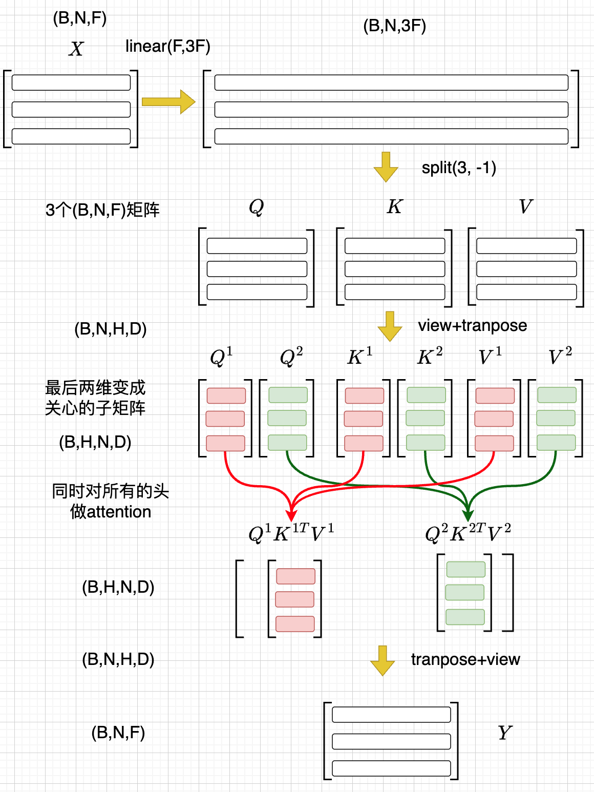
代码实现

 1
 2
 3
 4
 5
 6
 7
 8
 9
10
11
12
13
14
15
16
17
18
19
20
21
22
23
24
25
26
27
28
29
30
31
32
33
34
35
36
37

# 参考 https://github.com/karpathy/minGPT/tree/master/mingpt
import torch
import torch.nn as nn
import math
from torch.nn import functional as F

class SelfAttention(nn.Module):

  def __init__(self, config):
      super().__init__()
      self.H = config["n_head"]
      self.F = config["hidden_dim"] #F
      self.D = self.F // self.H #D
      # 一次把qkv 全部映射完成，对应W_Q, W_K, W_V
      self.qkv_proj = nn.Linear(self.F, 3 * self.F)
      # 最后的投影，对应于 $W_O$
      self.out_proj = nn.Linear(self.F, self.F)

  def forward(self, x):
      B, N, F = x.size()
      q, k, v = self.qkv_proj(x).split(self.F, dim=-1)
      # matmul 只能在最后两个维度相乘，需要对NxD的矩阵相乘，做1,2维度的交换
      k = k.view(B, N, self.H, self.D).transpose(1, 2)
      q = q.view(B, N, self.H, self.D).transpose(1, 2)
      v = v.view(B, N, self.H, self.D).transpose(1, 2)
      # (B,H,N,D)
      # 一次把多个头的映射全部完成, 对任意的(batch, head)
      att = (q @ k.transpose(-2, -1)) * (1.0 / math.sqrt(k.size(-1)))
      att = F.softmax(att, dim=-1)
      y = att @ v
      # (B,H,N,D)
      y = y.transpose(1, 2)
      # (B,N,H,D)
      # 最后两个维度合并
      y = y.contiguous().view(B, N, F)
      y = self.out_proj(y)
      return y

代码示意

位置无关的全连接

• 两层的全连接 \(\mathcal{F}(X_i)=(g(X_iW_1)+b_1)W_2+b_2\)

代码

 1
 2
 3
 4
 5
 6
 7
 8
 9
10
11

import torch
import torch.nn as nn
class PWiseFeedForward(nn.Module):
    def __init__(self, config):
        super().__init__()
        self.F = config["F"]
        self.proj_wide = nn.Linear(self.F, 4 * self.F)
        self.proj_narrow = nn.Linear(4 * self.F, self.F)
        self.act = nn.ReLU()
    def forward(self, x):
        return self.proj_narrow(self.act(self.proj_wide(x)))

归一化 + 残差网络

\(\mathcal{T}(X)=\mathcal{F}\circ\mathcal{A}(X)\)

Layer Normalization

\(\mathcal{A}’(X)=\mathcal{N}\circ\mathcal{A}(X)\) \(\dfrac{x-\mu}{\sqrt{\sigma}}\gamma + \beta,\mu=\dfrac{1}{d}\sum\limits_{i=1}^{d}x_{i}, \sigma=\sqrt{\dfrac{1}{d}\sum\limits_{i=1}^{d}(x_{i}-\mu)^{2}}\) 可以看成是作用在行向量上的算子

行归一化 or 列归一化

• 在NLP的序列建模里面，Layer Normalization
• 在CV/CTR预估里面, Batch Normalization

Why

• padding的影响 不同batch中<pad>个数不同，沿着token方向做归一化没有意义
• 每个位置做独立的归一化更有意义

• 输入矩阵例子

  \(\begin{pmatrix} \text{hello} \\ \text{world} \\ \text{pad} \\ \text{pad} \\ \text{pad} \end{pmatrix} \rightarrow X= \begin{pmatrix} [0.59, 0.20, 0.04, 0.96] \\ [0.96, 0.30, 0.16, 0.63] \\ [0.02, 0.19, 0.34, 0.25] \\ [0.02, 0.19, 0.34, 0.25] \\ [0.02, 0.19, 0.34, 0.25] \end{pmatrix}\)

其他的可能选择

• RMSNorm

  \(\dfrac{x}{\text{RMS}(x)}, \quad \text{RMS}(x) = \sqrt{\frac{1}{d} \sum_{i=1}^{d} x_i^2}\)

整体的变换

\(Y=\mathcal{T}(X)\)

1. Attention \(Z=\mathcal{N}\circ(X+\mathcal{A}(X))\)
2. 位置无关的全连接 \(Y=\mathcal{N}\circ(X+\mathcal{F}(Z))\)

residual network

\(\mathcal{A}’(X)=\mathcal{N}\circ(X+\mathcal{A}(X))\) \(\mathcal{F}’(X)=\mathcal{N}\circ(X+\mathcal{F}(X))\)

多层

一个 \(L\) 层的transformer 模型

\begin{equation*} \begin{split} \mathcal{T}(X) & = \mathcal{T}_L \circ \ldots \mathcal{T}_{2}\circ \mathcal{T}_{1}(X) \end{split} \end{equation*}

代码

 1
 2
 3
 4
 5
 6
 7
 8
 9
10
11
12
13
14

import torch.nn as nn
class Block(nn.Module):

    def __init__(self, config):
        super().__init__()
        self.layer_norm_1 = nn.LayerNorm(config["hiden_dim"])
        self.attn = SelfAttention(config)
        self.layer_norm_2 = nn.LayerNorm(config["hidden_dim"])
        self.mlp = PWiseFeedForward(config)

    def forward(self, x):
        x = self.layer_norm_1(x + self.attn(x))
        x = self.layer_norm_2(x + self.mlp(x))
        return x

transformer参数和计算量

关于参数量

• 一般的模型增加复杂度的方式
  • 增加深度，增加宽度
  • 增加embedding的维度
  • 增加词典的大小
• 各种dnn主要的参数位置
  • cnn: \(Y_{i}=(X_{i-1},X_i, X_{i+1}) W\)
  • rnn: \(Y_{i}=tanh(X_{i}W + Y_{i-1}U)\)

参数的分布

多头注意力 \(4F^2\)

• 每个头有
  • 3个投影矩阵 \(W_Q, W_K, W_V\)
  • 1个投影concat结果的矩阵 \(W_O\)
• 参数量: 假设投射到的子空间维度是\(D\), \(H\) 个子空间，\(D\times H = F\)
  • \(F\times D \times 3 \times H = 3F^{2}\)
  • \(F^{2}\)

FFW \(8F^2\)

• 两个矩阵，先从\(F\) 变宽到\(4F\)，再收窄回来到\(F\)
• 参数量\(F\times4F + 4F\times F= 8F^{2}\)

word embedding

\(E\) 是token字典的大小

• \(E\times F\)

total

\(L(12F^{2})+EF\)

linear transformer

两个算子的计算量

• \(\mathcal{A}(X)\) 计算量 \(O(N^2)\)
• \(\mathcal{F}(X)\) 计算量 \(O(N)\)

softmax 导致了\(O(N^2)\)

核心的计算量在这三个矩阵的相乘上，\(QK^{T}V\), 乘法的计算量密切依赖于矩阵组合的方式

• 有softmax的存在的话 只能先计算\(H=QK^{T}\), 对\(H\) 做softmax 变换后，再计算\(HV\) 乘法的计算量是 \(N^2D+N^2M\), 整体的复杂度是\(O(N^{2})\) \(QK^TV=(QK^T)V=\begin{pmatrix} H_{11},H_{12},\ldots,H_{1N} \\ \vdots\\ H_{N1},H_{N2},\ldots,H_{NN} \\ \end{pmatrix}V\)

• 如果没有softmax的话 可以先计算后两个矩阵相乘\(H=K^TV\), 再计算\(QH\) 乘法的计算量是 \(NDM+DMN=2NDM\)，当\(N\gg D\) 的时候, 计算量可以是\(O(N)\), \(K^TV\) 提前算出来缓存，大致如下面这个表达所示 \(Q(K^TV)=\begin{pmatrix} Q_1 \\ Q_2 \\ \vdots\\ Q_{N} \end{pmatrix}(K^TV)\)

kernel

\(\mathcal{A}(X_i)=\dfrac{\sum_{j=1}^{N} sim(Q_i,K_j) V_j}{\sum_{j=1}^N sim(Q_i,K_j)}\)

• kernel: \(k(x,y)=<\phi(x),\phi(y)>\) \(k(x,y)=(x\cdot z)^2, \phi(x)=(x_{1}^{2},x_{2}^2,\sqrt{2}x_1x_{2})\)
  • kernel 对应一个feature map
  • 可以用非负的kernel来替换掉
  • 当前的sim函数 \(sim(x,y)=\mathrm{exp}(xy^{T}/\sqrt{D})\)

linear transformer \(O(N)\)

• 用kernel来替换掉sim \[\begin{aligned}\mathcal{A}(X_i) &= \frac{\sum_{j=1}^{N} sim(Q_i,K_j) V_j}{\sum_{j=1}^N sim(Q_i,K_j)} \\ &=\frac{\sum_{j=1}^{N} \phi(Q_i)\phi(K_j)^T V_j}{\sum_{j=1}^N \phi(Q_i)\phi(K_j)^T} \\ &=\frac{ \phi(Q_i) \sum_{j=1}^{N}\phi(K_j)^T V_j}{\phi(Q_i)\sum_{j=1}^N \phi(K_j)^T} \end{aligned} \]
  • \(\sum_{j=1}^{N}\phi(K_j)^T V, \sum_{j=1}^N \phi(K_j)^T\) 可以提前算好
  • \(O(N)\) 复杂度，Linear Transformer
  • \(\phi(x)=\mathrm{elu}(x)+1\)

总结

• attention的设计原理解读
  • 从低阶语义向量到高阶语义向量的转化 \(\mathcal{T}\begin{pmatrix} X_1\\ X_2\\ \vdots\\ X_N \end{pmatrix} \rightarrow\begin{pmatrix} Y_1\\ Y_2\\ \vdots\\ Y_N \end{pmatrix}\)
  • \(\begin{aligned}\mathcal{A}(X_i) &= \frac{\sum_{j=1}^{N} sim(X_i,X_j) X_j}{\sum_{j=1}^N sim(X_i,X_j)} \end{aligned}\)
  • \(\mathcal{A}(X_i)=\dfrac{\sum_{j=1}^{N} sim(X_iW_Q,X_jW_{K}) X_jW_{V}}{\sum_{j=1}^N sim(X_iW_Q,X_jW_K)}\)
  • \(\begin{aligned}\mathcal{A}(X_i) &= \frac{\sum_{j=1}^{N} sim(Q_i,K_j) V_j}{\sum_{j=1}^N sim(Q_i,K_j)} \end{aligned}\)
• transformer的核心两次变换
  • \(Y=\mathcal{F}\circ \mathcal{A}(X)\) 做两次矩阵的变换
• 核心的计算量在这三个矩阵的相乘上，\(QK^{T}V\)
  • \((QK^T)V\) 计算量 \(O(N^2)\)
  • \(Q(K^TV)\) 计算量 \(O(N)\)
• linear transformer \[\begin{aligned}\mathcal{A}(X_i) &= \frac{\sum_{j=1}^{N} sim(Q_i,K_j) V_j}{\sum_{j=1}^N sim(Q_i,K_j)} \\ &=\frac{\sum_{j=1}^{N} \phi(Q_i)\phi(K_j)^T V_j}{\sum_{j=1}^N \phi(Q_i)\phi(K_j)^T} \\ &=\frac{ \phi(Q_i) \sum_{j=1}^{N}\phi(K_j)^T V_j}{\phi(Q_i)\sum_{j=1}^N \phi(K_j)^T} \end{aligned} \]

参考论文